News & Blogs

Decision Trees are very popular analytical tool used by business managers. Their popularity hinges upon their simple representation in terms of graphs and easy to implement as a set-of rules in the decision making process. Decision Trees have a tree-like graph of decisions and their possible consequences.  Decision Tree is a supervised machine learning algorithm, mostly used for classification problems where the output variables are binary or categorical. A supervised algorithm is one, where training data is analyzed to infer a function that can be used for mapping new data1. Typically supervised learning algorithm will calculate the error and back propagate the error in an iterative method to reduce error until it converges2. Trees are an excellent way to deal with complex decisions, which always involve many different factors and usually involve some degree of uncertainty3.

For example,  think about a classification problem where one has to decide who will play cricket from a sample of 30, based on three variables (or factors) – Gender (Male or Female), Class (IX, X), Height (<5.5 ft, >=5.5 ft). The variable that splits the sample into most homogeneous sets of students (i.e. sets being heterogeneous to each other) is the most significant variable. In the following display, Gender becomes the most significant variable, as it splits the sample into most homogeneous sets
       
       

Components of a Decision Tree –   

• The Decision, displayed as a square node with 2 or more arcs pointing to the options.


• The Event Sequence, displayed as a circle node (and are called sometimes as “chance nodes”) with 2 or more arcs pointing out the events; at times, probabilities may be displayed with the circle nodes.


• The Consequences or endpoint, also called as a “Terminal” and represented as a triangle, are the costs or utilities associated with different pathways.

Decision trees have a natural “if...then...else” construction, that makes them easier to fit into a programmatic structure6. They are best suited to categorization problems, where attributes or features are checked to arrive at a final category. For e.g., a decision tree can be used to effectively determine the species of an animal.

Decision trees owe their origin to ID3 (Iterative Dichotomiser 3) algorithm, which was invented by Ross Quinlan7. The ID3 algorithm uses the popular Entropy method to draw a decision tree, and this method is discussed in more detail in an upcoming blog on Random Forest. However, there came another algorithm called CHAID (Chi-square Automatic Interaction Detection), which was developed by Gordon Kass8, and which would help making the decision to select the order of choosing categorical predictors and branch the categories appropriately to form splits at each node, thus forming the decision tree. In the rest of this blog, I will take a shot at explaining Decision Trees formed by applying chi-square tests.

In a decision tree, the 1st step is that of feature (variable) selection in order to divide the tree at the very 1st level. This will require to calculate the chi-square value for all the predictors (if there are any continuous variables, they need to transform into categorical).

Let’s assume a dependent variable having d>=2 categories and a certain predictor variable in the analysis having p>= 2 categories.
       
       

A, B, C, D, E and F denote the observed values and EA, EB, EC, ED, EE and EF denote the expected values.

As the considered categories for this predictor variable are considered to be 3 significantly independent events, it can be said that probability of category p1 occurs in the positive class instances is equal to the probability that category p1 occurs in all the instances of the 2 classes9.

Thus, EA/ (A+C+E) = (A+B)/N

Or EA= M X (A+B)/N

Similarly, EB, EC, ED, EE and EF can be calculated.

Thereafter, we can calculate the chi-square test for this predictor variable as

 where, Ok and Ek are observed and expected values respectively and df is the degree of freedom. which is 2 [ i.e. (no. of categories in predictor variable – 1) X (no. of categories in dependent variable – 1)] in this case.

Let’s see how the above equation is constructed with the help of a sample data about gender distribution among various occupations in an area as follows.

Chi-square value for the Predictor called Occupation is
       
       = 1.819

 The predictor variable (say Xi) having the highest chi-square value will be selected to form the branch at a particular level of the decision tree
       
       

 The use of chi-square tests adds efficiency in the form of apt no. of splits for each categorical predictor. This method to split efficiently is called as CHAID. Suppose, while forming the decision tree, at a level of the decision tree, there is a predictor with maximum chi-square value. Hereafter, the following steps10 are undertaken to get the apt no. of splits using the predictor:

1. Cross-tabulate each predictor variable with the dependent variable and take steps 2 and 3    


2. For this predictor variable, find the allowable pair of categories whose (2 X categories in dependent variable) sub-table is least significantly different; if this significance level is below the critical level, merge these 2 categories and consider them as a compound category. Repeat this step


3. For each compound category, having more than 2 of original categories, find the most significant binary split and resolve the merger into a split if this significance level is beyond the critical level; in case a split happens, return to step 2


4. Calculate the Χ2or significance level for the optimally merged predictor; if this significance is greater than a criterion value, split the data at the merged categories of the predictorThe census data from UCI Machine Learning Repository is taken to explain the process above. Let’s just pick only the categorical independent variables (6; for simplicity, I have removed Country and gender variables) for this exercise. Snapshot of data is presented below. The data is used to predict whether someone makes over $50k a year (a positive event) or not (a negative event). 

 

The 1st step is that of feature selection by calculating the chi-square value for each predictor and choosing the predictor with highest value (relationship in this case).

Next step is to efficiently split the data at relationship level, i.e. choosing the right no. of categories. For this the significance test at stage of merging the categories will give the apt no. of branches – in this case, it is the combined categories of Husband with other non-Wife categories and Wife category as shown in the green portion below.

Thus, the 1st node of the tree would look like below.

Let’s show the split at Wife Node. We will follow the above mentioned steps to find the best feature and then optimize the split w.r.t. that feature, i.e. merge the allowable categories in the chosen predictor. The predictor occupation is selected at this node to split the sample collected at Wife Node. Various mentioned occupations are combined &colour-coded to form 4 groups – white collar jobs (white), blue collar jobs which need speciality (blue), jobs which don’t need much supervision (green) and others (grey).This grouping is done purely on my understanding for the purpose of this study and doesn’t intend to have bias of any sort; apologies, if there is any. After that, the categories of occupation predictor are combined to give an optimal split under the Wife Node.

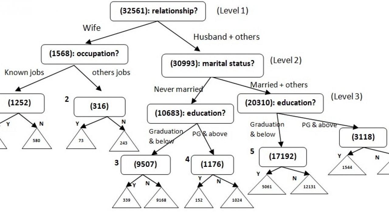
The tree is completed following the above steps for each node at all the levels. No. of levels, or the tree depth, can’t exceed no. of predictors in the data. Another stopping criterion is when the node is pure11 (i.e. only one category from the target or dependent variable is present in the node). Ideally, a decision tree should have max 3 or 4 levels – too many levels tend to make a tree over-fit (more on this one in the next blog on Random Forest) and hence biased during future predictions. Moreover, the nodes should have size greater than 3% (can also be set at 5%) of the entire training sample to be representing a decision node; otherwise, we stop any further division at that node.

Decision Trees are greedy algorithms, i.e. they have a tendency to over-fit. Hence, at times they need to undergo the process of Pruning12, which is a method to decrease the complexity of the classifier function, i.e. reduce the no. of features required to classify the training sample into one of the options from target variable. Caution is taken during the Pruning process to not affect the predictive accuracy of the decision tree. The complete Decision Tree formed from the above UCI data is shown below (level of the tree is 3).

       
 We will finish this blog by showing the efficiency of the Decision Tree, where we will compare its performance with a random generator (i.e. one where you guess 50% as positive and rest 50% as negative events from a sample). Considering each of the 6 nodes (as numbered above) as samples, we can plot a gain/lift chart and check the average lift from this algorithm.